6.6 卷积神经网络（LeNet）

LeNet，它是最早发布的卷积神经网络之一，因其在计算机视觉任务中的高效性能而受到广泛关注。 这个模型是由AT&T贝尔实验室的研究员Yann LeCun在1989年提出的（并以其命名），目的是识别图像 (LeCun et al., 1998)中的手写数字

当时，LeNet 取得了与支持向量机（support vector machines）性能相媲美的成果，成为监督学习的主流方法。 LeNet 被广泛用于自动取款机（ATM）机中，帮助识别处理支票的数字。时至今日，一些自动取款机仍在运行 Yann LeCun 和他的同事 Leon Bottou 在上世纪90年代写的代码

1. 网络结构

LeNet 中的数据流（都是 $X$ 的维度）。输入是手写数字，输出为10种可能结果的概率

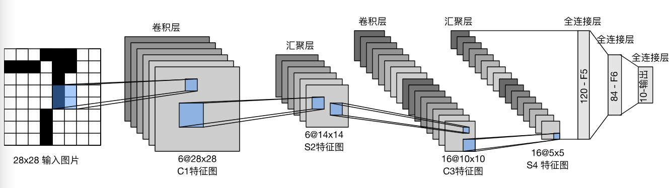
• 2 个卷积层组成：用来学习图片空间结构
• 2 个汇聚层：减少像素敏感度
• 3 个全连接层：转换到类别空间

2. 代码实现

2.1 模型定义

import torch
from torch import nn
from d2l import torch as d2l

net = nn.Sequential(                                            # 1x28x28
    nn.Conv2d(1, 6, kernel_size=5, padding=2), nn.Sigmoid(),    # 6x28x28
    nn.AvgPool2d(kernel_size=2, stride=2),                      # 6x14x14
    nn.Conv2d(6, 16, kernel_size=5), nn.Sigmoid(),              # 16x10x10
    nn.AvgPool2d(kernel_size=2, stride=2),                      # 16x5x5
    nn.Flatten(),                                               # 1x16*5*5
    nn.Linear(16 * 5 * 5, 120), nn.Sigmoid(),                   # 1x120
    nn.Linear(120, 84), nn.Sigmoid(),                           # 1x84
    nn.Linear(84, 10))                                          # 1x10

# 打印一下样本经过各个层的变化大小
X = torch.rand(size=(1, 1, 28, 28), dtype=torch.float32)
for layer in net:
    X = layer(X)
    print(layer.__class__.__name__,'output shape: \t',X.shape)

Conv2d output shape: 	 torch.Size([1, 6, 28, 28])
Sigmoid output shape: 	 torch.Size([1, 6, 28, 28])
AvgPool2d output shape: 	 torch.Size([1, 6, 14, 14])
Conv2d output shape: 	 torch.Size([1, 16, 10, 10])
Sigmoid output shape: 	 torch.Size([1, 16, 10, 10])
AvgPool2d output shape: 	 torch.Size([1, 16, 5, 5])
Flatten output shape: 	 torch.Size([1, 400])
Linear output shape: 	 torch.Size([1, 120])
Sigmoid output shape: 	 torch.Size([1, 120])
Linear output shape: 	 torch.Size([1, 84])
Sigmoid output shape: 	 torch.Size([1, 84])
Linear output shape: 	 torch.Size([1, 10])

2.2 模型训练

基本上与 3.6 softmax 回归的从零开始实现 一致，但在模型评估的时候，我们把数据搬到 GPU 上进行评估：

def evaluate_accuracy_gpu(net, data_iter, device=None): #@save
    """使用GPU计算模型在数据集上的精度"""
    if isinstance(net, nn.Module):
        net.eval()  # 设置为评估模式
        if not device:
            device = next(iter(net.parameters())).device
    # 正确预测的数量，总预测的数量
    metric = d2l.Accumulator(2)
    with torch.no_grad():
        for X, y in data_iter:
            if isinstance(X, list):
                # BERT微调所需的（之后将介绍）
                X = [x.to(device) for x in X]
            else:
                X = X.to(device)
            y = y.to(device)
            metric.add(d2l.accuracy(net(X), y), y.numel())
    return metric[0] / metric[1]

下面是训练与评估，注意网络搬到 GPU 与张量搬到 GPU 的不同 5.6 GPU#^0dfcd0

#@save
def train_ch6(net, train_iter, test_iter, num_epochs, lr, device):
    """用GPU训练模型(在第六章定义)"""
    def init_weights(m):
        if type(m) == nn.Linear or type(m) == nn.Conv2d:
            nn.init.xavier_uniform_(m.weight)
    net.apply(init_weights)
    print('training on', device)
    net.to(device)
    optimizer = torch.optim.SGD(net.parameters(), lr=lr)
    loss = nn.CrossEntropyLoss()
    animator = d2l.Animator(xlabel='epoch', xlim=[1, num_epochs],
                            legend=['train loss', 'train acc', 'test acc'])
    timer, num_batches = d2l.Timer(), len(train_iter)
    for epoch in range(num_epochs):
        # 训练损失之和，训练准确率之和，样本数
        metric = d2l.Accumulator(3)
        net.train()
        for i, (X, y) in enumerate(train_iter):
            timer.start()
            optimizer.zero_grad()
            X, y = X.to(device), y.to(device)
            y_hat = net(X)
            l = loss(y_hat, y)
            l.backward()
            optimizer.step()
            with torch.no_grad():
                metric.add(l * X.shape[0], d2l.accuracy(y_hat, y), X.shape[0])
            timer.stop()
            train_l = metric[0] / metric[2]
            train_acc = metric[1] / metric[2]
            if (i + 1) % (num_batches // 5) == 0 or i == num_batches - 1:
                animator.add(epoch + (i + 1) / num_batches,
                             (train_l, train_acc, None))
        test_acc = evaluate_accuracy_gpu(net, test_iter)
        animator.add(epoch + 1, (None, None, test_acc))
    print(f'loss {train_l:.3f}, train acc {train_acc:.3f}, '
          f'test acc {test_acc:.3f}')
    print(f'{metric[2] * num_epochs / timer.sum():.1f} examples/sec '
          f'on {str(device)}')

lr, num_epochs = 0.9, 10
train_ch6(net, train_iter, test_iter, num_epochs, lr, d2l.try_gpu())

loss 0.488, train acc 0.815, test acc 0.804 39314.0 examples/sec on cuda:0

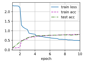
和 MLP 相比 4.3 多层感知机的简洁实现#^ca663a，卷积神经网络模型复杂度不高，所以没有发生过拟合, 还需要进一步微调（CNN 可以达到 0.95，深度学习中这个数字不是最关键的，最关键的是这个值是否达到用户需求），卷积神经网络最大的好处就是高维输入可以很好地学习，这个例子维度不算高，所以能用 MLP 学习

参考文献

• CNN 可视化的图形解释（好看，但没什么用）